Conditional formatting is an Excel feature you can use when you want to format cells based on their content. For example, you can have a cell turn red when it contains a number lower than 100. But how do you highlight an entire row?
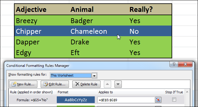
But what if you wanted to highlight other cells based on a cell’s value? The screenshot above shows some codenames used for Ubuntu distributions. One of these is made up; when I entered “No” in the “Really” column, the entire row got different background and font colors. To see how this was done, read on.
Creating Your Table
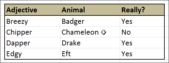
The first thing you will need is a simple table containing the data you’d like to format. The data doesn’t have to be text-only; you can use formulas freely. At this point, your table has no formatting at all:

Setting The Look-and-Feel
Now it’s time to format your table using Excel’s “simple” formatting tools. Format only those parts that won’t be affected by conditional formatting. In our case, we can safely set a border for the table, as well as format the header line. I’m going to assume you know how to do this part. You should end up with a table looking like this (or maybe a bit prettier):
Creating The Conditional Formatting Rules
And now we come to the meat and potatoes. As we said at the outset, if you’ve never used conditional formatting before, this might be a tad too much to begin with.
Select the first cell in the first row you’d like to format, click Conditional Formatting (in the Home tab) and select Manage Rules.

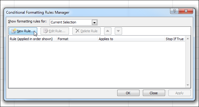
In the Conditional Formatting Rules Manager click New Rule.
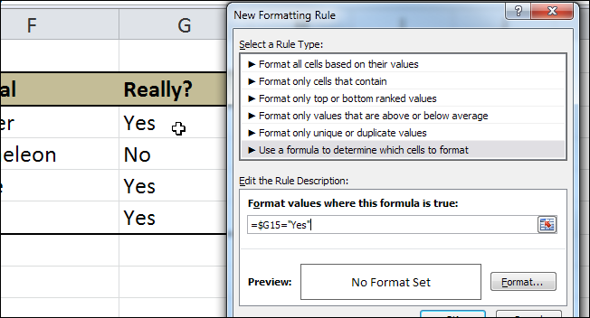
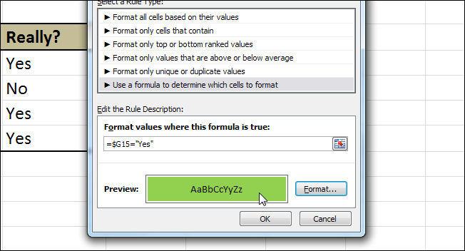
 In the New Formatting Rule dialog, click the last option – Use a formula to determine which cells to format. This is the trickiest part: Your formula must evaluate to “True” for the rule to apply, and must be flexible enough so you could use it across your entire table later on. Let’s analyze my sample formula:
=$G15 – this part is a cell’s address. G is the column which I want to format by (“Really?”). 15 is my current row. Note the dollar sign before the G – if I don’t have this symbol, when I apply my conditional formatting to the next cell, it would expect H15 to say “Yes”. So in this case, I need to have a “fixed” column ($G) but a “flexible” row (15), because I will be applying this formula across multiple rows.
=”Yes” – this part is the condition that has to be met. In this case we’re going for the simplest condition possible – it just has to say “Yes”. You can get very fancy with this part.
So in English, our formula is true whenever cell G in the current row has the word Yes in it.
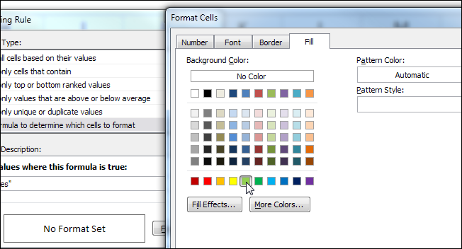
 Next, let’s define the formatting. Click the Format button. In the Format Cells dialog, go through the tabs and tweak the settings until you get the look you want. Here we’ll just be changing the fill to a different color.
 Once you’re got the desired look, click OK. You can now see a preview of your cell in the New Formatting Rule dialog.
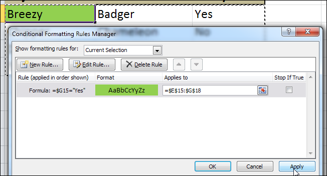
 Click OK again to get back to the Conditional Formatting Rules Manager and click Apply. If the cell you selected changes formatting, that means your formula was correct. If the formatting doesn’t change, you need to go a few steps back and tweak your formula until it does work.
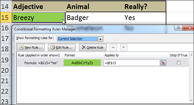 Now that we have a working formula, let’s apply it across our entire table. As you can see above, the formatting applies only to the cell we started off with. Click the button next to the Applies to field and drag the selection across your entire table.
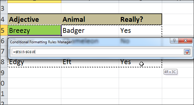 Once done, click the button next to the address field to get back to the full dialog. You should still see a marquee around your entire table, and now the Applies to field contains a range of cells and not just a single address. Click Apply.
Every row in your table should now be formatted according to the new rule:
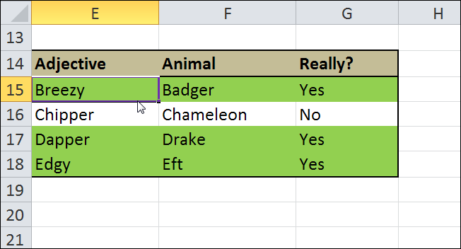 That’s it! Now all you have to do is create another rule to format rows that say “No”.